NumPy library allows us to perform various operations which needs to be done on data structures often used in Machine Learning and Data Science like vectors, matrices and arrays. We will only show most common operations with NumPy which are used in a lot of Machine Learning pipelines. Finally, please note that NumPy is just a way to perform the operations, so, the mathematical operations we show are the main focus of this lesson and not the NumPy package itself. Let’s get started.
What is a Vector?
According to Google, a Vector is a quantity having direction as well as magnitude, especially as determining the position of one point in space relative to another.

Vectors are very important in Machine Learning as they not just describe magnitude but also the direction of the features. We can create a vector in NumPy with following code snippet:
row_vector = np.array([1,2,3])
print(row_vector)
In the above code snippet, we created a row vector. We can also create a column vector as:
col_vector = np.array([[1],[2],[3]])
print(col_vector)
Making a Matrix
A matrix can be simply understood as a two-dimensional array. We can make a matrix with NumPy by making a multi-dimensional array:
print(matrix)
Although matrix is exactly similar to multi-dimensional array, the matrix data structure is not recommended due to two reasons:
- The array is the standard when it comes to the NumPy package
- Most of the operations with NumPy returns arrays and not a matrix
Using a Sparse Matrix
To remind, a sparse matrix is the one in which most of the items are zero. Now, a common scenario in data processing and machine learning is processing matrices in which most of the elements are zero. For example, consider a matrix whose rows describe every video on Youtube and columns represents each registered user. Each value represents if the user has watched a video or not. Of course, majority of the values in this matrix will be zero. The advantage with sparse matrix is that it doesn’t store the values which are zero. This results in a huge computational advantage and storage optimisation as well.
Let’s create a spark matrix here:
original_matrix = np.array([[1, 0, 3], [0, 0, 6], [7, 0, 0]])
sparse_matrix = sparse.csr_matrix(original_matrix)
print(sparse_matrix)
To understand how the code works, we will look at the output here:

In the above code, we used a NumPy’s function to create a Compressed sparse row matrix where non-zero elements are represented using the zero-based indexes. There are various kinds of sparse matrix, like:
- Compressed sparse column
- List of lists
- Dictionary of keys
We won’t be diving into other sparse matrices here but know that each of their is use is specific and no one can be termed as ‘best’.
Applying Operations to all Vector elements
It is a common scenario when we need to apply a common operation to multiple vector elements. This can be done by defining a lambda and then vectorizing the same. Let’s see some code snippet for the same:
[1, 2, 3],
[4, 5, 6],
[7, 8, 9]])
mul_5 = lambda x: x * 5
vectorized_mul_5 = np.vectorize(mul_5)
vectorized_mul_5(matrix)
To understand how the code works, we will look at the output here:
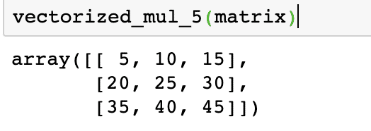
In the above code snippet, we used vectorize function which is part of the NumPy library, to transform a simple lambda definition into a function which can process each and every element of the vector. It is important to note that vectorize is just a loop over the elements and it has no effect on the performance of the program. NumPy also allows broadcasting, which means that instead of the above complex code, we could have simply done:
And the result would have been exactly the same. I wanted to show the complex part first, otherwise you would have skipped the section!
Mean, Variance and Standard Deviation
With NumPy, it is easy to perform operations related to descriptive statistics on vectors. Mean of a vector can be calculated as:
Variance of a vector can be calculated as:
Standard deviation of a vector can be calculated as:
The output of the above commands on the given matrix is given here:

Transposing a Matrix
Transposing is a very common operation which you will hear about whenever you are surrounded by matrices. Transposing is just a way to swap columnar and row values of a matrix. Please note that a vector cannot be transposed as a vector is just a collection of values without those values being categorised into rows and columns. Please note that converting a row vector to a column vector is not transposing (based on the definitions of linear algebra, which is outside the scope of this lesson).
For now, we will find peace just by transposing a matrix. It is very simple to access the transpose of a matrix with NumPy:
The output of the above command on the given matrix is given here:

Same operation can be performed on a row vector to convert it to a column vector.
Flattening a Matrix
We can convert a matrix into a one-dimensional array if we wish to process its elements in a linear fashion. This can be done with the following code snippet:
The output of the above command on the given matrix is given here:
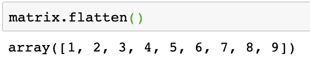
Note that the flatten matrix is a one-dimensional array, simply linear in fashion.
Calculating Eigenvalues and Eigenvectors
Eigenvectors are very commonly used in Machine Learning packages. So, when a linear transformation function is presented as a matrix, then X, Eigenvectors are the vectors that change only in scale of the vector but not its direction. We can say that:
Here, X is the square matrix and γ contains the Eigenvalues. Also, v contains the Eigenvectors. With NumPy, it is easy to calculate Eigenvalues and Eigenvectors. Here is the code snippet where we demonstrate the same:
The output of the above command on the given matrix is given here:

Dot Products of Vectors
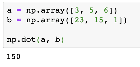
Dot Products of Vectors is a way of multiplying 2 vectors. It tells you about how much of the vectors are in the same direction, as opposed to the cross product which tells you the opposite, how little the vectors are in the same direction (called orthogonal). We can calculate the dot product of two vectors as given in the code snippet here:
b = np.array([23, 15, 1])
np.dot(a, b)
The output of the above command on the given arrays is given here:
Adding, Subtracting and Multiplying Matrices
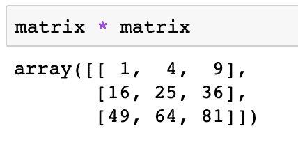
Adding and Subtracting multiple matrices is quite straightforward operation in matrices. There are two ways in which this can be done. Let’s look at the code snippet to perform these operations. For the purpose of keeping this simple, we will use the same matrix twice:
Next, two matrices can be subtracted as:
The output of the above command on the given matrix is given here:
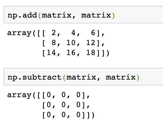
As expected, each of the elements in the matrix is added/subtracted with the corresponding element. Multiplying a matrix is similar to finding the dot product as we did earlier:
The above code will find the true multiplication value of two matrices, given as:
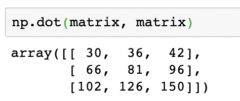
The output of the above command on the given matrix is given here:
Conclusion
In this lesson, we went through a lot of mathematical operations related to Vectors, Matrices and Arrays which are commonly used Data processing, descriptive statistics and data science. This was a quick lesson covering only the most common and most important sections of the wide variety of concepts but these operations should give a very good idea about what all operations can be performed while dealing with these data structures.
Please share your feedback freely about the lesson on Twitter with @linuxhint and @sbmaggarwal (that’s me!).